
Architecture and components#
Datasets in MOMA#
MOMA works with two primary types of data objects: rasters and maps.
Raster Objects#
Raster objects store raw data values on a regular grid for a specific site, together with metadata describing spatial resolution and geographic location.
MOMA supports the following raster types:
RasterMono
A single-band raster containing raw digital values.RasterRGBA
A four-band raster where data is stored as RGBA color values.
To process this data in MOMA, a value map is used to convert colors into labels or numeric values.
Uncertainty Encoding#
Both raster types support additional bands to encode uncertainty. In all cases, the primary raster bands (one or four) represent the mean values.
Supported uncertainty representations are:
Single additional band
Encodes the standard deviation.Multiple additional bands
Each band encodes a single deviation from the mean. This option is used when the data distribution must be controlled outside MOMA.
Map Objects#
Map objects are used to process raster data in MOMA. Each map object:
Contains a raster dataset as described above
Provides map-specific functionality for data processing and visualization
Each map type is described in the next section.
MOMA Core Functionality#
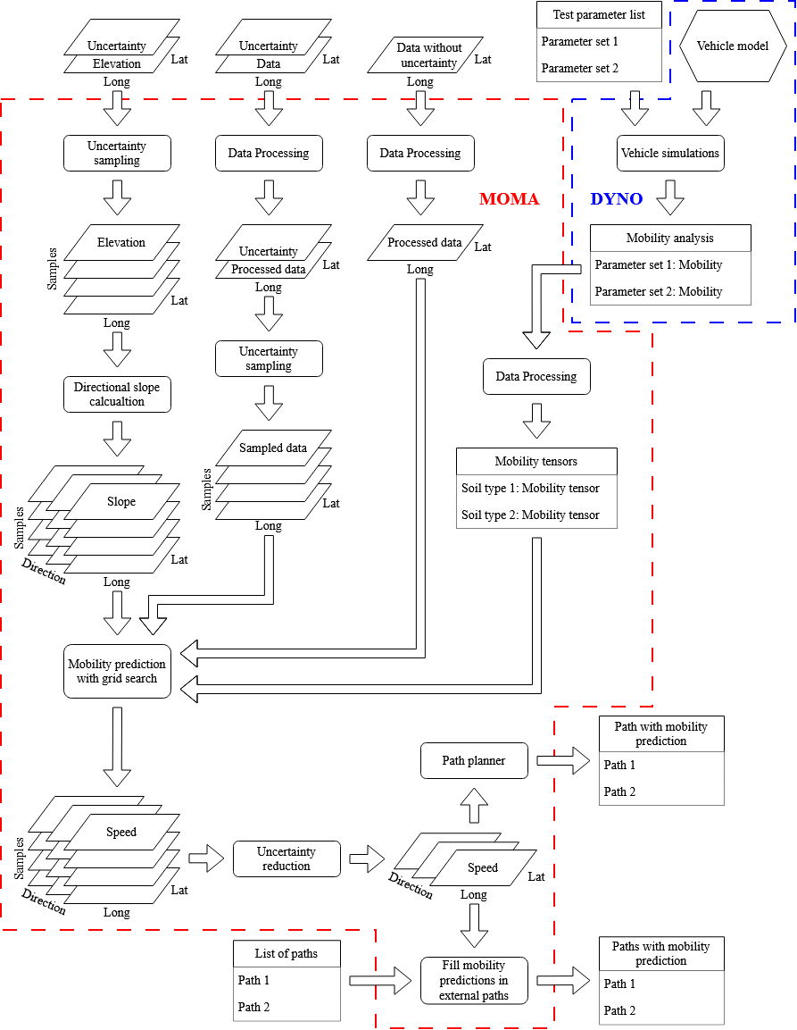
MOMA operates on a sequence of map objects, where each object represents a specific stage in the processing pipeline. The map objects are listed below in the order in which they are used.
If a map includes uncertainty information, (N) samples are drawn from the map’s distribution using Latin Hypercube Sampling.
This diagram shows how data is handled inside MOMA and DYNO from input to output
Aerial Map#
The aerial map provides a visual reference of the site and is primarily used as
the background layer for the no-go map. It is loaded as a RasterRGBA object,
which contains the raw color data required for aerial visualization.
Elevation Map#
The elevation map represents the ground elevation of the site. It is loaded as a
RasterMono object and may include additional bands that encode uncertainty in
the elevation data.
Directional Slope Map#
For each sample drawn from the elevation map, a set of directional slope maps is generated—one for each of the eight primary compass directions. Slopes are computed using aspect and the steepest slope direction.
To avoid errors at the map boundaries, the elevation map is padded with values computed using forward differences toward the edges. To reduce local errors caused by noise, the resulting slope maps are smoothed by averaging each local value with the mean of a 3×3 kernel centered at that point.
The directional slope maps are stored as RasterMono objects.
Soil Map#
The soil type map specifies the soil type present at each location. Soil type is used as an input parameter for generating the mobility maps. The map is loaded as a RasterRGBA, where each soil type is represented by a distinct color. These colors are converted into soil type labels using a value map. For visualization, the colors are taken directly from the raster.
Moisture Map#
The moisture map represents the moisture content at each location within the site. Similar to soil type, moisture is used as an input parameter when generating the mobility maps.
The moisture map is loaded as a RasterRGBA object, where a colormap with
discrete moisture levels is encoded directly in the raster. Additional bands
may be included to represent uncertainty in the moisture data. The raster
colors are converted to numerical moisture values using a value map. For
visualization, the original raster colors are used directly in the plots.
Friction Map#
The friction map defines the coefficient of friction for hard terrain at each
location. It is loaded as a RasterMono object and may include additional bands
that encode uncertainty in the friction values.
No-go Map#
The no-go map identifies areas where vehicle traversal is prohibited. It is constructed from two sources of information:
user-defined no-go zones specified in the
site.yamlfile, andland-use data combined with the vehicle-specific
landuse_nogo.yamlfile, which defines which land-use types are considered no-go for the vehicle in question.
User-defined no-go zones can be specified either as rectangular regions (defined by the coordinates of their edges) or as circular regions (defined by a center point and a radius).
For visualization, the no-go map is plotted using the aerial map as a background. User-defined no-go zones are shown in red, while land-use–based no-go zones are shown in orange.
Directional Mobility Map#
Using the maps described above, a set of directional mobility maps is generated.
For each soil type, a mobility tensor is created based on simulations from a
multibody vehicle model. These simulations evaluate vehicle mobility over a
finite set of parameter combinations which are stored in the used vehicles mobility.yaml file.
The finite set of simulated parameters defines a grid search, which allows mobility to be evaluated over a continuous parameter space. To populate the mobility maps, each grid cell is evaluated using the mobility tensor associated with its corresponding soil type. If a grid cell lies within a no-go zone, the mobility value is set to zero.
Although all parameters are parsed into the grid search, each soil type uses only a subset of these parameters. To handle this, each mobility tensor includes a mask that selects the relevant parameters. At present, only hard terrain has been evaluated, where mobility depends on slope and friction. In future work, soft terrain models may be added, in which moisture replaces friction as a key parameter.
This process produces a set of mobility maps for each sampled realization of the input data. The resulting sample space is reduced to a single set of mobility maps using a specified reduction function. The simplest reduction method is the arithmetic mean of all samples. Alternatively, a quantile-based reduction may be used—for example, a 90% quantile map represents mobility values that are met or exceeded with 90% probability.
Omnidirectional Mobility Map#
When the direction omni is used for mobility prediction, MOMA add an omnidirectional mobility map, where mobility is assumed to be identical in all directions. The process begins by averaging the absolute slope over the eight directions. A mobility map is then constructed in the same manner as the directional mobility map, but using the omnidirectional slope map instead of directional slope maps. Finally, mobility prediction based on the omnidirectional mobility map is carried out in the same way as in the directional case.
Path planning and traverse mobility prediction#
MOMA includes a built-in path planning module that uses generated mobility maps to compute a path between two locations. The planner is based on the A* algorithm, which minimizes a path cost defined over a grid representation of the environment.
The mobility maps are converted into a graph, where each cell is a node and edges connect neighboring cells. Each edge is assigned a weight that reflects the difficulty of traversing from one cell to another in a given direction.
To account for uncertainty in mobility predictions and to discourage traversal through low-mobility areas, MOMA uses a penalized cost formulation. The edge weight is computed as a power-law inverse of the predicted mobility:
Where:
\(Mobility[i, j, dir]\) is the predicted mobility for cell \((i, j)\) in the given travel direction.
\(p\) is a user-defined exponent \((p > 1)\) that increases the penalty for low mobility values.
\(ε\) is a small constant used to handle no-go or zero-mobility areas.
\(f(dir)\) is a directional scaling factor that accounts for longer distances when moving diagonally between cells.
This formulation intentionally penalizes low-mobility areas more strongly than a simple inverse relationship. While the resulting path cost no longer has a direct physical interpretation (such as travel time), it provides increased robustness when mobility estimates are uncertain.
By amplifying the cost of low-mobility regions, the path planner is biased toward safer, more traversable terrain. This reduces the risk of selecting paths where the vehicle could become stuck due to errors or uncertainty in the mobility maps, even if the predicted traversal time is longer.
Traverse Mobility Prediction#
Once a path has been defined, MOMA uses the generated mobility maps to predict mobility along the path. The vehicle is assumed to move in straight lines from the center of one grid cell to the center of the next.
For each segment of the path, MOMA computes and appends the following metrics:
Travel direction to the next cell
Slope in the direction of travel
Side slope
Predicted mobility for the current cell in the travel direction
Estimated traverse time to the next cell based on the predicted mobility
Accumulated travel time and distance along the path
These metrics provide a detailed estimate of the vehicle’s expected performance along the selected route and are computed using mobility values derived from both directional and omnidirectional mobility maps.
Importing Predefined Paths#
As an alternative to automatic path planning, MOMA supports mobility prediction for predefined paths using the --path_folder argument (see Section 2.1). This argument specifies a directory containing one or more path definitions.
Using predefined paths is useful in two main scenarios:
Controlled evaluation – It allows full control over which path is used, enabling systematic testing of mobility predictions in specific scenarios.
Comparative analysis – It enables comparison of predicted mobility across different inputs, parameters, or algorithmic changes without the path itself being altered by the path planner.